The Biot-Savart law

According to above as

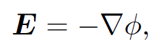
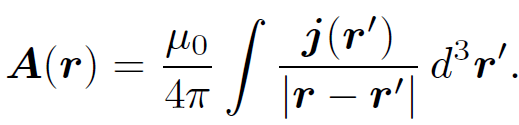
we can obtain an expression for the electric field generated by stationary charges by taking minus the gradient of

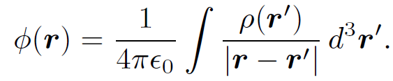
This yields

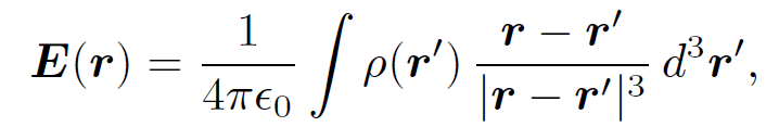 (1.1)

which we recognize as Coulomb's law written for a continuous charge distribution. According to above as

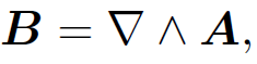
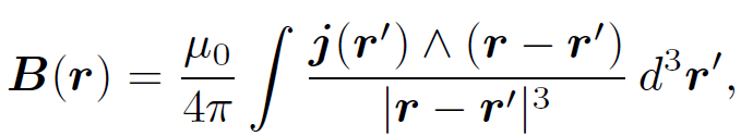
we can obtain an equivalent expression for the magnetic field generated by steady currents by taking the curl of

This gives

 (1.2)

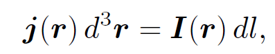
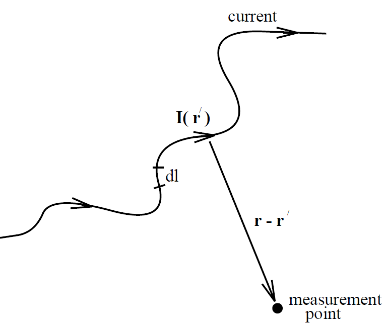
where use has been made of the vector identity ∇ ˄ (ϕA) = ϕ∇ ˄ A + ∇ϕ ˄ A. Equation (1.2) is known as the ''Biot-Savart law" after the French physicists Jean Baptiste Biot and Felix Savart; it completely specifies the magnetic field generated by a steady (but otherwise quite general) distributed current. Let us reduce our distributed current to an idealized zero thickness wire. We can do this by writing

 (1.3)

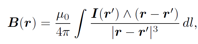
where I is the vector current (i.e., its direction and magnitude specify the direction and magnitude of the current) and dl is an element of length along the wire. Equations (1.2) and (1.3) can be combined to give

 (1.4)

which is the form in which the Biot-Savart law is most usually written. This

law is to magnetostatics (i.e., the study of magnetic fields generated by steady currents) what Coulomb's law is to electrostatics (i.e., the study of electric fields generated by stationary charges). Furthermore, it can be experimentally verified given a set of currents, a compass, a test wire, and a great deal of skill and patience. This justifies our earlier assumption that the field above as

are valid for general current distributions (recall that we derived them by studying the fields generated by infinite, straight wires). Note that both Coulomb's law and the Biot-Savart law are ''gauge independent"; i.e., they do not depend on the particular choice of gauge. Consider (for the last time!) an infinite, straight wire directed along the z-axis and carrying a current I. Let us reconstruct the magnetic field generated by

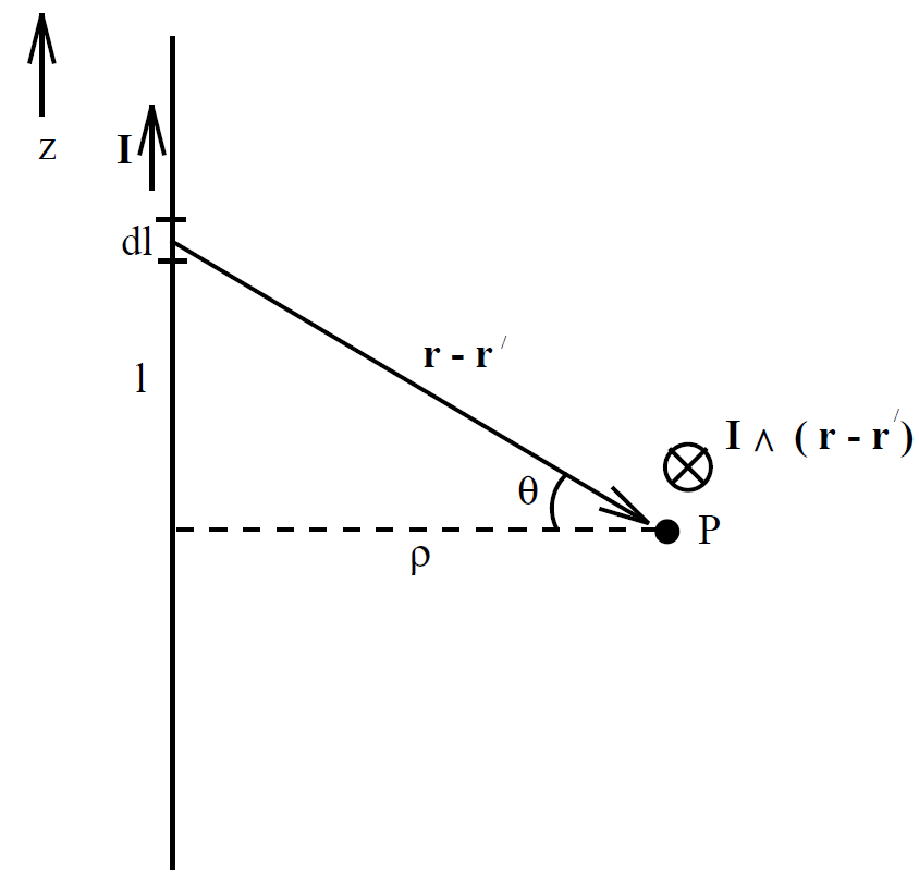
the wire at point P using the Biot-Savart law. Suppose that the perpendicular distance to the wire is ρ. It is easily seen that

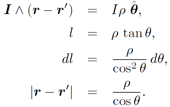 (1.5)

Thus, according to Eq. (1.4) we have

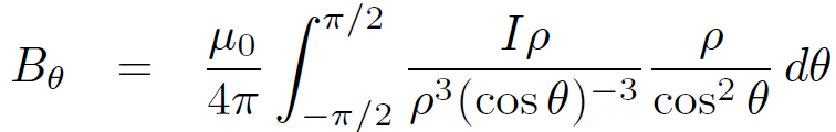
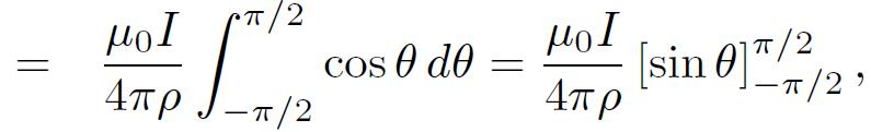  (1.6)

which gives the familiar result

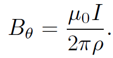 (1.7)

So, we have come full circle in our investigation of magnetic fields. Note that the simple result (1.7) can only be obtained from the Biot-Savart law after some non-trivial algebra. Examination of more complicated current distributions using this law invariably leads to lengthy, involved, and extremely unpleasant calculations.

مواضيع ذات صلة

The dipole radiator

Radiation

Electromagnetism

ثنائيات الأشعة السينية آلية عملها

انفجار الأشعة السينية المنبعثة من 1–Sco X

أستاذ المناطيد (مناطيد استكشاف الاشعة السينية)

استعادة التلسكوب الخاص باستكشاف الاشعة السينية من وسط الصحراء: جاك صائد حيوانات الكنغر

التحليق عاليا المناطيد.. وكواشف الأشعة السينية.. وعملية الإطلاق

مطاردة الأشعة السينية بالمناطيد.. البداية

ما هي الأشعة السينية؟

أشعة سينية من الفضاء الخارجي

إنجاز ماكسويل العظيم