تاريخ الفيزياء
علماء الفيزياء


الفيزياء الكلاسيكية
الميكانيك
الديناميكا الحرارية
الكهربائية والمغناطيسية
الكهربائية
المغناطيسية
الكهرومغناطيسية
علم البصريات
تاريخ علم البصريات
الضوء
مواضيع عامة في علم البصريات
الصوت
الفيزياء الحديثة
النظرية النسبية
النظرية النسبية الخاصة
النظرية النسبية العامة
مواضيع عامة في النظرية النسبية
ميكانيكا الكم
الفيزياء الذرية
الفيزياء الجزيئية
الفيزياء النووية
مواضيع عامة في الفيزياء النووية
النشاط الاشعاعي
فيزياء الحالة الصلبة
الموصلات
أشباه الموصلات
العوازل
مواضيع عامة في الفيزياء الصلبة
فيزياء الجوامد
الليزر
أنواع الليزر
بعض تطبيقات الليزر
مواضيع عامة في الليزر
علم الفلك
تاريخ وعلماء علم الفلك
الثقوب السوداء
المجموعة الشمسية
الشمس
كوكب عطارد
كوكب الزهرة
كوكب الأرض
كوكب المريخ
كوكب المشتري
كوكب زحل
كوكب أورانوس
كوكب نبتون
كوكب بلوتو
القمر
كواكب ومواضيع اخرى
مواضيع عامة في علم الفلك
النجوم
البلازما
الألكترونيات
خواص المادة
الطاقة البديلة
الطاقة الشمسية
مواضيع عامة في الطاقة البديلة
المد والجزر
فيزياء الجسيمات
الفيزياء والعلوم الأخرى
الفيزياء الكيميائية
الفيزياء الرياضية
الفيزياء الحيوية
الفيزياء والفلسفة
الفيزياء العامة
مواضيع عامة في الفيزياء
تجارب فيزيائية
مصطلحات وتعاريف فيزيائية
وحدات القياس الفيزيائية
طرائف الفيزياء
مواضيع اخرى

Black hole data
 المؤلف:
Heino Falcke and Friedrich W Hehl
المؤلف:
Heino Falcke and Friedrich W Hehl
 المصدر:
THE GALACTIC BLACK HOLE Lectures on General Relativity and Astrophysics
المصدر:
THE GALACTIC BLACK HOLE Lectures on General Relativity and Astrophysics
 الجزء والصفحة:
p 188
الجزء والصفحة:
p 188
 29-1-2017
 2467
2467


+
-
20
Black hole data
Horizons
By black hole data we understand vacuum data which contain apparent horizons. The informal definition of an apparent horizon is that it is the boundary of a trapped region, which means that its orthogonal outgoing null rays must have zero divergence. (Inside the trapped region they converge for any two-surface, by the definition of a ‘trapped region’.) The Penrose-Hawking singularity theorems state that the existence of an apparent horizon implies that the evolving spacetime will be singular (assuming the strong energy condition). Given also the condition that singularities cannot be seen by observers far off, a condition usually called cosmic censorship, one infers the existence of an event horizon and hence a black hole. One can then show that the intersection of the event horizon with the spatial hypersurface lies on or outside the apparent horizon (for stationary spacetimes they coincide). The reason why one does not deal with event horizons directly is that one cannot tell whether one exists by just looking at initial data. In principle one would have to evolve them to the infinite future, which is beyond our abilities in general. In contrast, apparent horizons can be recognized once the data on an initial slice are given. The formal definition of an apparent horizon is the following: given initial data (Σ, hi j , Ki j ) and an embedded two-surface σ ⊂ Σ with outward pointing normal νi , σ is an apparent horizon if and only if the following relation between Ki j , the extrinsic curvature of Σ in spacetime, and ki j , the extrinsic curvature of σ in Σ, is satisfied,
 (1.1)
(1.1)
where qi j := hi j −νiν j is just the induced Riemannian metric on σ, so that (1.1) simply says that the restriction of Ki j to the tangent space of σ has opposite trace to ki j . (The minus sign on the right-hand side of (1.1) signifies a future apparent horizon corresponding to a black hole which has a future event horizon. A plus sign would signify a past apparent horizon corresponding to a ‘white hole’ with past event horizon.) This means that once we have the data (Σ, hi j , Ki j ) we can in principle find all two-surfaces σ ⊂ Σ for which (1.1) holds and therefore find all apparent horizons.
Poincare charges
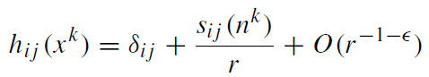
By Poincar'e charges we shall understand quantities like mass, linear momentum, and angular momentum. In GR they are associated with an asymptotic Poincar'e symmetry, provided that the data (Σ, hi j , Ki j ) are asymptotically flat in a suitable sense, which we will now explain. Topologically asymptotic flatness means that the non-trivial ‘topological features’ of Σ should all reside in a bounded region and not ‘pile up’ at infinity. More formally this is expressed by saying that there is a bounded region B ⊂ Σ such that Σ − B (the complement of B) consists of a finite number of disjoint pieces, each of which looks topologically like the complement of a ball in R3 . These asymptotic pieces are also called the ends of the manifold Σ. Next comes the geometric restriction imposed by the condition of asymptotic flatness. It states that for each end there is an asymptotically Euclidean coordinate system {x1, x2, x3} in which the fields (hi j , Ki j ) have the following fall-off for r →∞(r =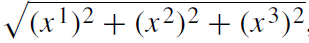 nk = xk/r ):
 (1.1)
(1.1)
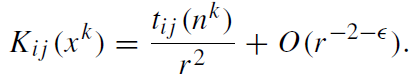 (1.2)
(1.2)
Moreover, in order to have convergent expressions for physically relevant quantities, like, e.g., angular momentum, the field si j must be an even function of its argument, i.e. si j (-nk ) = si j (nk ), and ti j must be an odd function, i.e. ti j (-nk ) = -ti j (nk ).
Under these conditions each end can be assigned mass, momentum, and angular momentum, which are conserved during time evolution. They may be computed by integrals over two-spheres in the limit that the spheres are pushed to larger and larger radii into the asymptotically flat region of that end. These so called ADM integrals (first considered by Arnowitt, Deser, and Misner) are given by the following expressions, which we give in ‘geometric’ units (meaning that in order to get them in standard units one has to multiply the mass expression given below by 1/κ and the linear and angular momentum by c/κ):
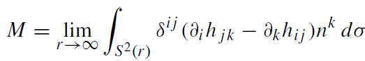 (1.3)
(1.3)
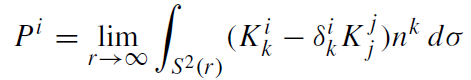 (1.4)
(1.4)
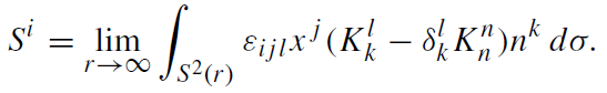 (1.5)
(1.5)
Maximal and time-symmetric data
The constraints:
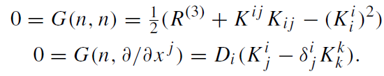
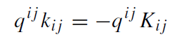
are too complicated to be solved in general. Further conditions are usually imposed to reduce the complexity of the problem: data (hi j , Ki j) are called maximal if Kii= hi j Ki j = 0. The name derives from the fact that Kii= 0 is the necessary and sufficient condition for a hypersurface to have a stationary volume to first order with respect to deformations in the ambient spacetime. Even though stationarity does not generally imply extremality, one calls such hypersurfaces maximal. Note also that since spacetime is a Lorentzian manifold, extremal spacelike hypersurfaces will be of maximal rather than minimal volume. In contrast, in Riemannian manifolds one would speak of minimal surfaces.
A much stronger condition is to impose Ki j = 0 which, implies that all momenta and angular momenta vanish. Only the mass is now allowed to be non-zero. Such data are called time symmetric since for them hi j is momentarily static. This implies that the evolution of such data into the future and into the past will coincide so that the developed spacetime will have a time-reversal symmetry which pointwise fixes the initial surface where Ki j = 0. This surface is therefore also called the moment of time symmetry. Time-symmetric data can still represent configurations of any number of black holes without angular momenta which are momentarily at rest. Note also that for time-symmetric data, for an apparent horizon is equivalent to the tracelessness of the extrinsic curvature of σ. Hence for time symmetric data apparent horizons are minimal surfaces.
We add one more general comment concerning submanifolds. A vanishing extrinsic curvature is equivalent to the property that each geodesic of the ambient space, which starts on, and tangent to the submanifold, will always run entirely inside the submanifold. Therefore, submanifolds with vanishing extrinsic curvature are called totally geodesic. Now, if the ambient space allows for an isometry (symmetry of the metric), whose fixed-point set is the submanifold in question, as for the time-reversal transformation just discussed, the submanifold must necessarily be totally geodesic. To see this, consider a geodesic of the ambient space which starts on, and tangent to the submanifold. Assume that this geodesic eventually leaves the submanifold. Then its image under the isometry would again be a geodesic (since isometries always map geodesics to geodesics) which is different from the one from which we started. But this is impossible since they share the same initial conditions which are known to determine the geodesic uniquely. Hence the geodesic cannot leave the submanifold, which proves the claim. We will later have more opportunities to identify totally geodesic submanifolds namely apparent horizons by their property of being fixed point sets of isometries.
Solution strategy for maximal data
Possibly the most popular approach to solving the constraints is the conformal technique due to York et al. The basic idea is to regard the Hamiltonian as an equation for the conformal factor of the metric hi j and freely specify the complementary information, called the conformal equivalence class of hi j . More concretely, this works as follows:
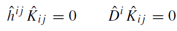
(1) Choose unphysical (‘hatted’) quantities (ĥ i j , ˆKi j ), where ĥi j is a Riemannian metric on Σ and ˆKi j is symmetric, trace and divergence free:
 (1.6)
(1.6)
where ˆD is the covariant derivative with respect to ĥ i j .
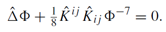
(2) Solve the (quasilinear elliptic) equation for a positive, real valued function Φ with boundary condition Φ (r →∞) →1, where ˆΔ = ĥ i j ˆDi
 (1.7)
(1.7)
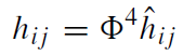
(3) Using the solution of (1.7), define physical (‘unhatted’) quantities by
 (1.8)
(1.8)
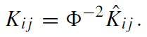 (1.9)
(1.9)
Explicit time-symmetric data
Before we say a little more about maximal data, we wish to present some of the most popular examples for time symmetric data some of which are also extensively used in numerical simulations. Hopefully these examples let you gain some intuition into the geometries and topologies involved and also let you anticipate the richness that a variable space structure gives to the solution space of one of the simplest equations in physics: the Laplace equation.
Restricting the solution strategy, outlined earlier, to the time-symmetric case, one first observes that for Ki j = 0 one has ˆK i j = 0. Which now simply becomes the Laplace equation for the single scalar function on the Riemannian manifold (Σ, ĥi j ).
We now make a further simplifying assumption, namely that ĥ i j is, in fact, the flat metric. This will restrict our solution hi j to a conformally flat geometry. It is not obvious how severe the loss of physically interesting solutions is by restricting ourselves to conformally flat metrics. But we will see that the latter already contain many interesting and relevant examples.
So let us solve Laplace's equation in flat space! Remember that Φ must be positive and approach one at spatial infinity (asymptotic flatness). We cannot take Σ = R3 since the only solution to the Laplace equation in R3 which asymptotically approaches one is identically one. We must allow to blow up at some points, which we can then remove from the manifold. In this way we let the solution tell us what topology to choose in order to have an everywhere regular solution. You might think that just removing singular points would be rather cheating, since the resulting manifold may turn out to be incomplete, that is, can be hit by a curve after finite proper length (you can go ‘there’), even though Φ and hence the physical metric blows up at this point. If this were the case, one would definitely have to say what a solution on the completion would be. But, as a matter of fact, this cannot happen and the punctured space will turn out to be complete in terms of the physical metric.
1.1 One black hole
The simplest solution with one puncture (at r = 0) is just
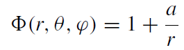 (1.10)
where a is a constant which we soon interpret and which must be positive in order for Φ to be positive everywhere. We cannot have other multipole contributions since they inevitably would force Φ to be negative somewhere. What is the geometry of this solution? The physical metric is
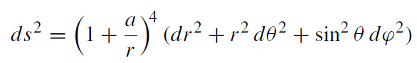 (1.11)
which is easily checked to be invariant under the inversion transformation on the sphere r = a:
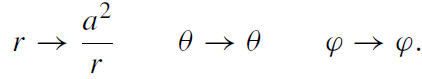 (1.12)
This means that the region r > a just looks like the region r < a and that the sphere r = a has the smallest area among all spheres of constant radius. It is a minimal surface, in fact even a totally geodesic submanifold, since it is the fixed point set of the isometry (1.12). Hence it is an apparent horizon, whose area follows from (1.11):
A = 16π(2a)2. (1.13)
Our manifold thus corresponds to a black hole (figure 1.1). Its mass can easily be computed; one finds m = 2a. This manifold has two ends, one for r → ∞and one for r → 0. They have the same geometry and hence the same ADM mass, as must be the case since individual and total mass clearly coincide for a single hole.
The data just written down correspond to the ‘middle’ slice right across the Kruskal (maximally extended Schwarzschild) manifold. Also, (1.11) is just the spatial part of the Schwarzschild metric in isotropic coordinates. Hence we know
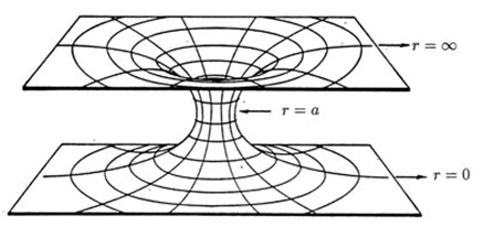
Figure 1.1. One black hole.
its entire future development in analytic form. Already for two holes this is no longer the case. Even the simplest two-body problem head on collision has not been solved analytically in GR.
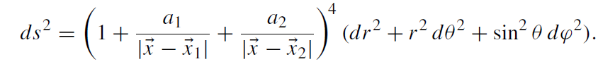
1.2 Two black holes
There is an obvious generalization of (1.10) by allowing two ‘monopoles’ of strength a1 and a2 at the punctures  = 1 and = 2 respectively. The three metric then reads:
 (1.14)
The manifold has now three asymptotically flat ends, one for |  | → ∞, where the overall ADM mass M is measured, and one each for | - 1,2| → 0. To see the latter, it is best to write the metric (1.14) in spherical polar coordinates (r1, θ1, ϕ1) centered at 1, and then introduce the inverted radial coordinate given by -r1 = a21/r1. In the limit -r1→∞, the metric then takes the form
 (1.15)
where r12 = | 1 - 2|. This looks just like a one-hole metric (1.11). Hence, if the black holes are well separated (compared to their size), the two-hole geometry looks like that depicted in figure 1.2. By comparison with the one hole metric, we can immediately write down the ADM masses corresponding to the three ends r, ‑r1,2→∞respectively:
 (1.16)
Momenta and angular momenta clearly vanish (moment of time symmetry). Still assuming well-separated holes, i.e. χi = ai/r12 << 1, we can calculate the
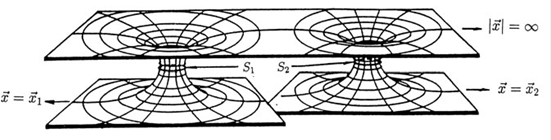
Figure 1.2. Two black holes well separated.
binding energy ΔE = M - m1 − m2 as a function of the masses mi and r12 and get
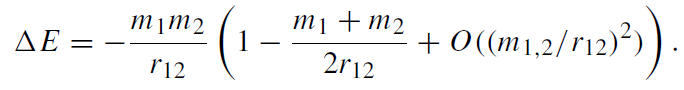 (1.17)
The leading order is just the Newtonian expression for the binding energy of two point particles with masses m1,2 at distance r12. But there are corrections to this Newtonian form which tend to diminish the Newtonian value. Note also that (1.17) is still not in a good form since r12 is not an invariantly defined geometric distance measure. As such one might use the length ! of the shortest geodesic joining the two apparent horizons S1 and S2. Unfortunately these horizons are not easy to locate analytically and hence no closed form of ℓ(m1,m2, r12) exists which could be inverted to eliminate r12 in favour of ℓ.
Due to the difficulty of locating the two apparent horizons analytically, we also cannot write down an analytic expression for their area. But we can give upper and lower bounds as follows:
 (1.18)
The lower bound simply follows from the fact that the two hole metric (1.14), if written down in terms of spherical polar coordinates about any of its punctures, equals the one-hole metric (1.11) plus a positive definite correction. The upper bound follows from the so-called Penrose inequality in Riemannian geometry, which directly states that 16πm2 ≥ A for each asymptotically flat end, where m is the mass and A is the area of the outermost minimal surface.
If the two holes approach each other to within a distance comparable to the sizes of the holes, the geometry changes in an essential way. This is shown in figure 1.3. The most important new feature is that new minimal surfaces form, in fact two, which both enclose the two holes. The outermost of these, as seen from the upper end, denoted by S3 in figure 1.3, corresponds to the apparent horizon of the newly formed ‘compound’ black hole which contains the two old ones. For two black holes of equal mass, i.e. a1 = a2 = a, this happens approximately for a parameter ratio of a/r12 = 0.65 which, in an approximate
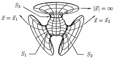
Figure 1.3. Two black holes after merging.
numerical translation into the ratio of individual hole mass to geodesic separation, reads m/ℓ ≈ 0.26.
1.3 More than two black holes
The method can be generalized in a straightforward manner to any number n of black holes with parameters (ai , i ), i = 1, . . . n, for the punctures. The manifold Σ has now n+1 ends, one for | | →∞and one for each → i . The expressions for the metric and masses are then given by the obvious generalizations of (1.14) and (1.16), respectively.
1.4 Energy bounds from Hawking’s area law
Loosely speaking, Hawking's area law states that the surface of a black hole cannot decrease with time. Let us briefly explain this statement. If Σ is a Cauchy surface (a spacelike hypersurface in spacetime) and H the event horizon (a lightlike hypersurface in spacetime), the two intersect in a number of components (spacelike two-manifolds), each of which we assume to be a two sphere. Each such two-sphere is called the surface of a black hole at time Σ. Let us pick one of them and call it B. Consider next a second Cauchy surface Σ' which lies to the future of Σ. The outgoing null rays of B intersect Σ' in a surface B', and the statement is now that the area of B' is larger than or equal to the area of B (to prove this one must assume the strong energy condition). Note that we deliberately left open the possibility that B' might be a proper subset of a black hole surface at time Σ', in case the original hole has merged in the meantime with another one. If this does not happen B' may be called the surface of the same black hole at the later time Σ.
This can be applied to the future evolution of multi black hole data as follows. As we have already mentioned, the event horizon lies on or outside the apparent horizon. Hence the area of the ‘surface’ (as just defined) of a black hole is bounded below by the area of the corresponding apparent horizon, which in turn has the lower bound stated in (1.18). Suppose that, after a long time, our configuration settles into an approximately stationary state, at least for some interior region where gravitational radiation is no longer emitted. Since our data have zero linear and angular momentum, the final state is static and uniquely given by a single Schwarzschild hole of some final mass Mfinal and corresponding surface area Afinal = 16πM2final. This is a direct consequence of known black hole uniqueness theorems. By the area theorem Afinal is not less than the sum of all initial apparent horizon surface areas. This immediately gives
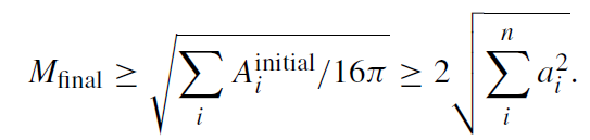 (1.19)
In passing we remark that applied to a single black hole this argument shows that it cannot lose its mass below the value mir :=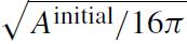 , called its irreducible mass. Back to the multi-hole case, the total initial mass is given by the straightforward generalization of (1.16):
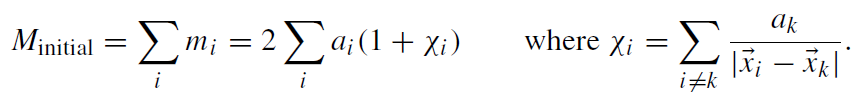 (1.20)
By using these two equations, we can write down a lower bound for the fractional energy loss into gravitational radiation:
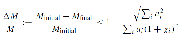 (1.21)
For a collision of n initially widely separated (χi → 0) holes of equal mass this becomes
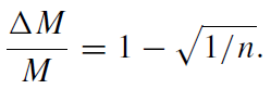 (1.22)
For just two holes this means that at most 29% of their total rest mass can be radiated away. But this efficiency can be enhanced if the energy is distributed over a larger number of black holes.
Another way to raise the upper bound for the efficiency is to consider spinning black holes. For two holes the maximal value of 50% can be derived by starting with two extremal black holes (i.e. of maximal angular momentum: J = m2 in geometric units) which merge to form a single unspinning black hole.
One can also envisage a situation where one hole participates in a scattering process but does not merge. Rather it gets kicked out of the collision zone and settles without spin (for simplicity) in a quasistationary state (for some time) far apart. The question is what fraction of energy the area theorem allows it to lose. Let this be the kth hole. Then mfinalk ≥ 2ak = minitialk /(1 + χk). Hence
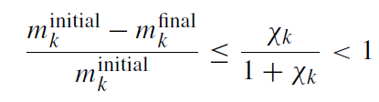 (1.23)
showing that an appreciable efficiency can only be obtained if the data are such that χk is not too close to zero. This means that the kth hole was originally not too far from the others. This seems an unlikely process. Hence it is difficult to extract energy from a single unspinning hole.
For a single spinning black hole the situation is again different. Spinning it down from an extreme state to zero angular momentum sets an upper bound for the efficiency from the area law of 29%. This follows easily from the following relation between mass, irreducible mass, and angular momentum for a Kerr black hole:
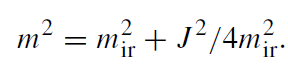 (1.24)
Setting J = m2, one solves for mir/m = √1/2; hence (m − mir)/m =1 −√1/2 ≈ 0.29. It can, moreover, that this limit can be (theoretically) realized by the Penrose process.
Needless to say, realistic processes may be far less efficient than this theoretical bound from the area law alone indicates. Recent numerical studies of the head on (i.e. zero angular momentum) collision of two equal-mass black holes give a radiated energy in units of the total energy of only 10−3. With angular momentum the efficiency is, of course, expected to be much better. Here recent numerical investigations give an estimate of 3 × 10⁻² for an inspiralling of two equal-mass non-spinning black holes from the innermost stable circular orbit : still a long way from the theoretical upper bound.
1.5 Other topologies
Other topologies can be found which support initial data with apparent horizons. For example, instead of the ‘Schwarzschild’ manifold with n +1 ends for n black holes (figure 1.4), one can find one which has just two ends for any number ≥ 2 of holes and which has been termed the Einstein–Rosen manifold (figure 1.5). The difference from the data already discussed does not primarily lie in the physics they represent. After all their different topologies are hidden behind event horizons for the outside observer, even though their interaction energies are slightly. However, the point we wish to stress here is that such data can analytically and numerically be more convenient, despite the fact that the underlying manifold might seem topologically more complicated. The reason is that these data have more symmetries and that coordinate systems can be found for which these symmetries take simple analytic expressions. For example, in the Einstein-Rosen manifold the upper and lower ends are isometrically related
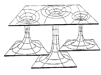
Figure 1.4. Multi-Schwarzschild.
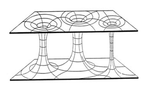
Figure 1.5. Einstein–Rosen manifold.
by reflections about the minimal two-spheres in each connecting tube, with the fixed point sets being the apparent horizons. Hence all the apparent horizons can be easily located analytically in the multi-hole Einstein-Rosen manifold, in contrast to the multi-hole Schwarzschild manifold.
Let us briefly explain this for two holes of equal mass. Here one starts again from R3 coordinatized by spherical bipolar coordinates. These are obtained from bipolar coordinates (μ, η) in the xz-plane by adding an azimuthal angle φ corresponding to a rotation about the z-axis, just as ordinary spherical polar coordinates are produced from ordinary polar coordinates in the xz-plane. The coordinates (μ, η) parametrize the xz-plane according to exp(μ − iη) = (ξ + c)/ (ξ − c), where ξ = z + i x and c > 0 is a constant (figure 1.6). The lines of constant μ intersect those of constant η orthogonally. Both families consist of circles; those in the first family are centered on the z-axis with radii c/ sinhμ at z = c cothμ, and those in the second family on the x-axis with radii c/ | sin η| at |x| = c cot η.
Following an idea of Misner's, one can borrow the method of images from electrostatics in order to construct solutions Φ to the Laplace equation such that the metric hi j = Φ4δi j has a number of reflection isometries about two-spheres, one for each hole. In the two-hole case, one uses the two two-spheres μ = ±μ0 for some μ0 > 0, which then become the apparent horizons. By using these isometries, we can take two copies of our
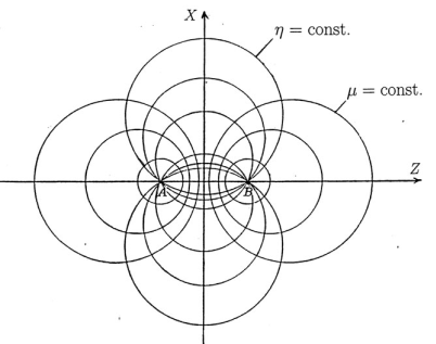
Figure 1.6. Bipolar coordinates.
initial manifold, excise the balls |μ| > μ0 and glue the two remaining parts ‘back to back’ along the two boundaries μ = μ0 and μ = −μ0. The isometry property is necessary so that the metric continues to be smooth across the seam. This gives an Einstein-Rosen manifold with two tubes (or ‘bridges’, as they are sometimes called) connecting two asymptotically flat regions.
In fact, we could have just taken one copy of the original manifold, excised the balls |μ| > μ0, and mutually glued together the two boundaries μ = ±μ0. This also gives a smooth metric across the seam and results in a manifold known as the Misner wormhole (figure 1.7). Metrically the Misner wormhole is locally isometric to the Einstein-Rosen manifold with two tubes (which is its ‘double cover’), but their topologies obviously differ. This means that for the observer outside the apparent horizons, these two data sets are indistinguishable. This is not quite true for the Einstein-Rosen and Schwarzschild data, which are not locally isometric. Even without exploring the region inside the horizons (which anyway is rendered impossible by existing results on topological censorship) they slightly differ in their interaction energy and other geometric quantities, e.g. the tidal deformation of the apparent horizons.
The two parameters c and μ0 now label the two hole configurations of equal mass. (In the Schwarzschild case the two independent parameters were
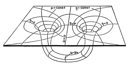
Figure 1.7. The Misner wormhole representing two black holes.
a ≡ a1 = a2 and r12 ≡| 1 - 2|.) But unlike the Schwarzschild case, we can now give closed analytic expressions not only for the total mass M and individual mass m in terms of the two parameters, but also for the geodesic distance of the apparent horizons ℓ. (ℓ is used as the definition for the ‘instantaneous distance of the two black holes’; for the Misner wormhole, where the two apparent horizons are identified, this corresponds to the length of the shortest geodesic winding once around the wormhole.) These read:
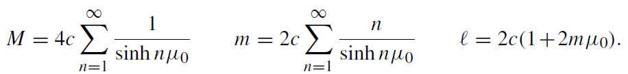 (1.25)
You might rightly wonder what ‘individual mass’ should be if there is no internal end associated with each black hole where the ADM can be applied. The answer is that there are alternative definitions of ‘quasi-local mass’ which can be applied even without asymptotic ends. The one we previously used for the expression of m is due and is easy to compute in connection with the method of images but it lacks a deeper mathematical foundation. An alternative which is mathematically better founded, which, however, is much harder to calculate and only applies to a limited set of situations (it agrees with the ADM mass whenever both definitions apply). Amongst them are, however, all time-symmetric conformally flat data, and for data above the Penrose mass has fortunately. The expression for m is rather complicated and differs from that given here. The difference is only of sixth order in an expansion in (mass/distance).
In summary, we see that the problem of setting up initial data for two black holes of given individual mass and given separation has no unique answer. Metrically as well as topologically different data sets can be found which have the same right to be called a realization of such a configuration. For holes without associated asymptotically flat ends no unambiguous definition for a quasi-local
 الاكثر قراءة في الثقوب السوداء
 اخر الاخبار
اخبار العتبة العباسية المقدسة

الآخبار الصحية


مواضيع ذات صلة
 قسم الشؤون الفكرية يصدر كتاباً يوثق تاريخ السدانة في العتبة العباسية المقدسة
 "المهمة".. إصدار قصصي يوثّق القصص الفائزة في مسابقة فتوى الدفاع المقدسة للقصة القصيرة
 (نوافذ).. إصدار أدبي يوثق القصص الفائزة في مسابقة الإمام العسكري (عليه السلام)