Retarded potentials

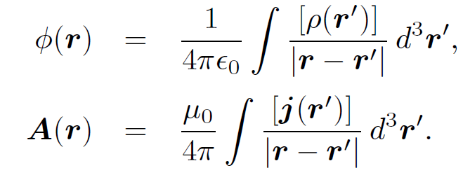
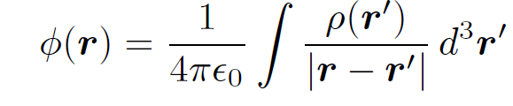
We are now in a position to solve Maxwell's equations. Recall that in steady state Maxwell's equations reduce to

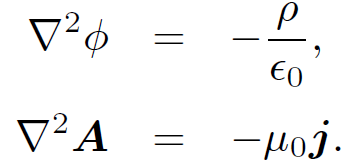 (1.1)

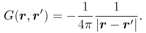
The solutions to these equations are easily found using the Green's function for Poisson's above as:

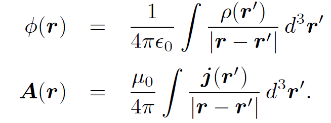 (1.2)

The time dependent Maxwell equations reduce to

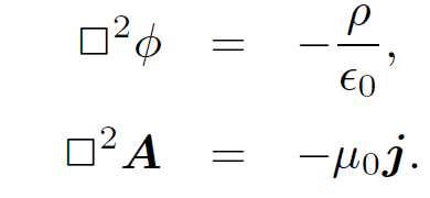 (1.3)

We can solve these equations using the time dependent Green's

.

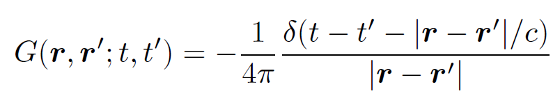From above as

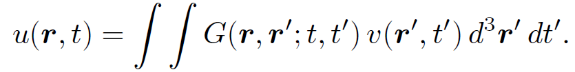
we find that

 (1.4)

with a similar equation for A. Using the well known property of delta functions, these equations reduce to

 (1.5)

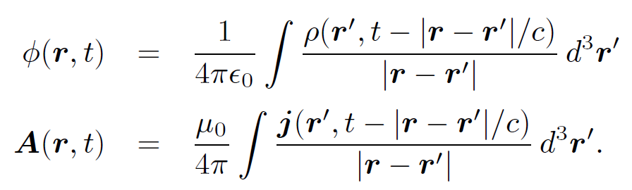
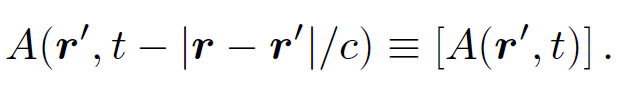
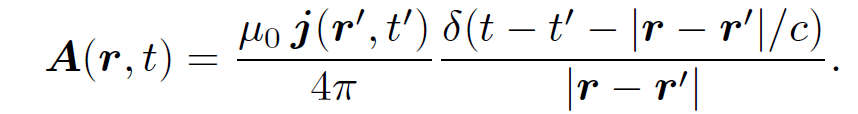
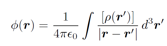
These are the general solutions to Maxwell's equations! Note that the time dependent solutions (1.5) are the same as the steady state solutions (1.2), apart from the weird way in which time appears in the former. According to Eqs. (1.5), if we want to work out the potentials at position r and time t we have to perform integrals of the charge density and current density over all space (just like in the steady state situation). However, when we calculate the contribution of charges and currents at position rʹ to these integrals we do not use the values at time t, instead we use the values at some earlier time t-|r-rʹ|/c. What is this earlier time? It is simply the latest time at which a light signal emitted from position rʹ would be received at position r before time t. This is called the retarded time. Likewise, the potentials (1.5) are called retarded potentials. It is often useful to adopt the following notation

 (1.6)

The square brackets denote retardation (i.e., using the retarded time instead of the real time). Using this notation Eqs. (1.5) become

 (1.7)

The time dependence in the above equations is taken as read. We are now in a position to understand electromagnetism at its most fundamental level. A charge distribution ρ(r, t) can thought of as built up out of a collection or series of charges which instantaneously come into existence, at some point rʹ and some time tʹ, and then disappear again. Mathematically, this is written

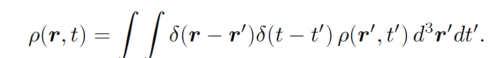 (1.8)

Likewise, we can think of a current distribution j(r, t) as built up out of a collection or series of currents which instantaneously appear and then disappear:

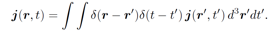 (1.9)

Each of these ephemeral charges and currents excites a spherical wave in the appropriate potential. Thus, the charge density at rʹ and tʹ sends out a wave in the scalar potential:

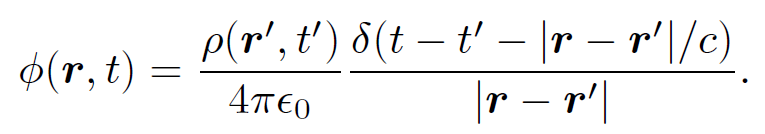 (1.10)

Likewise, the current density at rʹ and tʹ sends out a wave in the vector potential:

 (1.11)

These waves can be thought of as little messengers which inform other charges and currents about the charges and currents present at position rʹ and time tʹ. However, the messengers travel at a finite speed; i.e., the speed of light. So, by the time they reach other charges and currents their message is a little out of date. Every charge and every current in the universe emits these spherical waves. The resultant scalar and vector potential fields are given by Eqs. (1.7). Of course, we can turn these fields into electric and magnetic fields using Eqs. (1.8). We can then evaluate the force exerted on charges using the Lorentz formula. We can see that we have now escaped from the apparent action at a distance nature of Coulomb's law and the Biot-Savart law. Electromagnetic information is carried by spherical waves in the vector and scalar potentials and, therefore, travels at the velocity of light. Thus, if we change the position of a charge then a distant charge can only respond after a time delay sufficient for a spherical wave to propagate from the former to the latter charge. Let us compare the steady-state law

 (1.12)

with the corresponding time dependent law

 (1.13)

These two formulae look very similar indeed, but there is an important difference. We can imagine (rather pictorially) that every charge in the universe is continuously performing the integral (1.12), and is also performing a similar integral to find the vector potential. After evaluating both potentials, the charge can calculate the fields and using the Lorentz force law it can then work out its equation of motion. The problem is that the information the charge receives from the rest of the universe is carried by our spherical waves, and is always slightly out of date (because the waves travel at a finite speed). As the charge considers more and more distant charges or currents its information gets more and more out of date. (Similarly, when astronomers look out to more and more distant galaxies in the universe they are also looking backwards in time. In fact, the light we receive from the most distant observable galaxies was emitted when the universe was only about a third of its present age.) So, what does our electron do? It simply uses the most up to date information about distant charges and currents which it possesses. So, instead of incorporating the charge density ρ(r, t) in its integral the electron uses the retarded charge density [ρ(r, t)] (i.e., the density evaluated at the retarded time). This is effectively what Eq. (1.13) says.

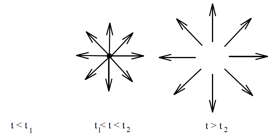
Consider a thought experiment in which a charge q appears at position rʹ at time t₁, persists for a while, and then disappears at time t₂. What is the electric field generated by such a charge? Using Eq. (1.13), we find that

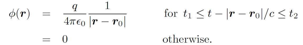 (1.14)

Now, E = - ∇ ϕ (since there are no currents, and therefore no vector potential is generated), so

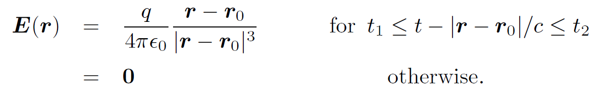 (1.15)

This solution is shown pictorially above. We can see that the charge effectively emits a Coulomb electric field which propagates radially away from the charge at the speed of light. Likewise, it is easy to show that a current carrying wire effectively emits an Amperian magnetic field at the speed of light. We can now appreciate the essential difference between time dependent electromagnetism and the action at a distance laws of Coulomb and Biot & Savart. In the latter theories, the field lines act rather like rigid wires attached to charges (or circulating around currents). If the charges (or currents) move then so do the field lines, leading inevitably to unphysical action at a distance type behaviour. In the time dependent theory charges act rather like water sprinklers; i.e., they spray out the Coulomb field in all directions at the speed of light. Similarly, current carrying wires throw out magnetic field loops at the speed of light. If we move a charge (or current) then field lines emitted beforehand are not affected, so the field at a distant charge (or current) only responds to the change in position after a time delay sufficient for the field to propagate between the two charges (or currents) at the speed of light. In Coulomb's law and the Biot-Savart law it is not

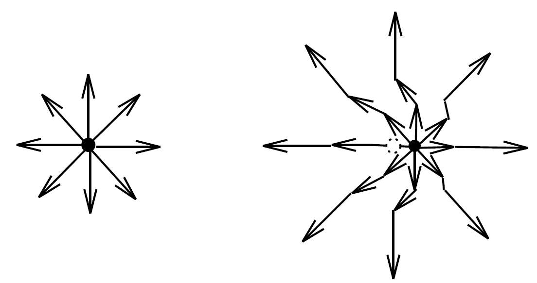
obvious that the electric and magnetic fields have any real existence. The only measurable quantities are the forces acting between charges and currents. We can describe the force acting on a given charge or current, due to the other charges and currents in the universe, in terms of the local electric and magnetic fields, but we have no way of knowing whether these fields persist when the charge or current is not present (i.e., we could argue that electric and magnetic fields are just a convenient way of calculating forces but, in reality, the forces are trans-mitted directly between charges and currents by some form of magic). However, it is patently obvious that electric and magnetic fields have a real existence in the time dependent theory. Consider the following thought experiment. Suppose that a charge q₁ comes into existence for a period of time, emits a Coulomb field, and then disappears. Suppose that a distant charge q₂ interacts with this field, but is sufficiently far from the first charge that by the time the field arrives the first charge has already disappeared. The force exerted on the second charge is only ascribable to the electric field; it cannot be ascribed to the first charge because this charge no longer exists by the time the force is exerted. The electric field clearly transmits energy and momentum between the two charges. Anything which possesses energy and momentum is ''real" in a physical sense. Later on in this course we shall demonstrate that electric and magnetic fields conserve energy and momentum. Let us now consider a moving charge. Such a charge is continually emitting spherical waves in the scalar potential, and the resulting wave front pattern is sketched below. Clearly, the wave fronts are more closely spaced in front of the

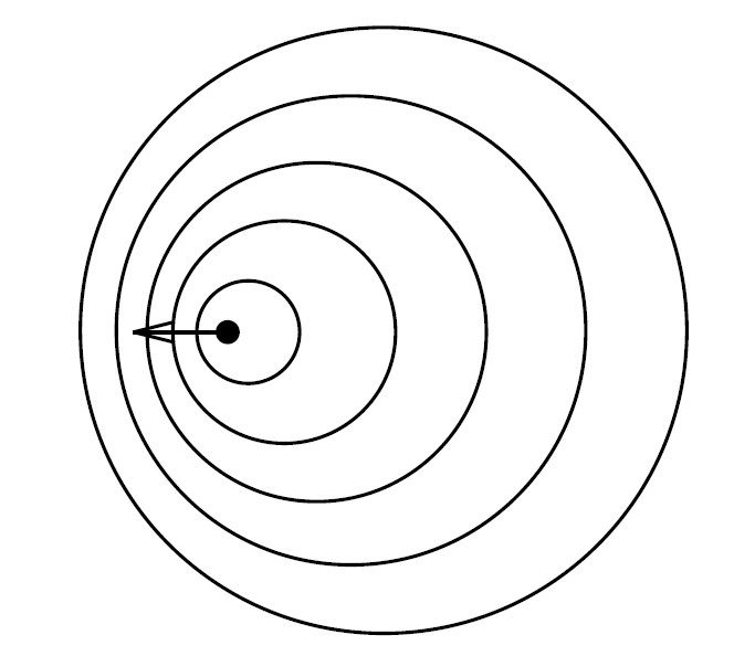
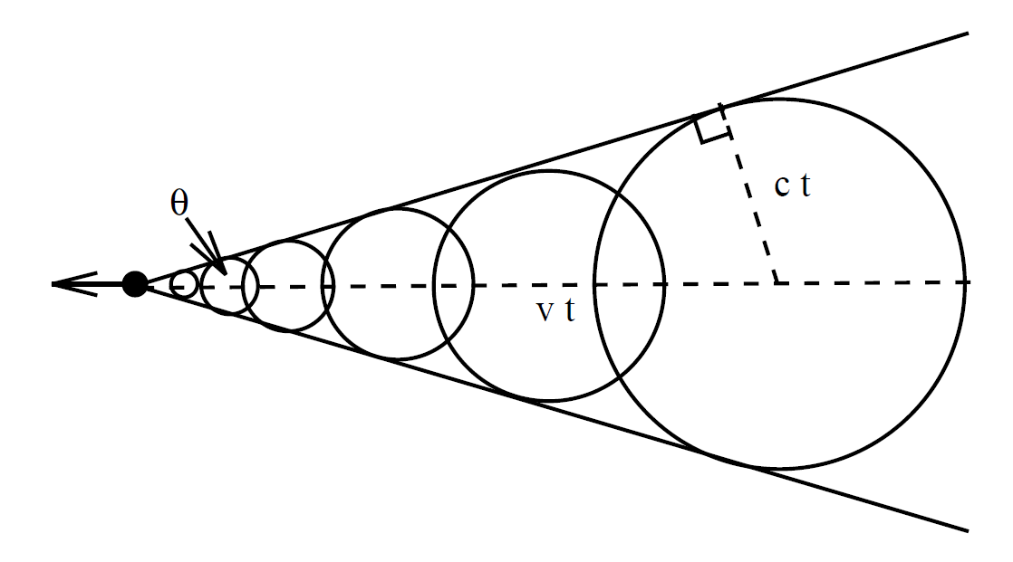
charge than they are behind it, suggesting that the electric field in front is larger than the field behind. In a medium, such as water or air, where waves travel at a finite speed c (say) it is possible to get a very interesting effect if the wave source travels at some velocity v which exceeds the wave speed. This is illustrated below. The locus of the outermost wave front is now a cone instead of a sphere. The wave intensity on the cone is extremely large: this is a shock wave! The half angle θ of the shock wave cone is simply cos^-1(c/v). In water, shock waves are produced by fast moving boats. We call these ''bow waves." In air, shock waves are produced by speeding bullets and supersonic jets. In the latter case we call  these ''sonic booms." Is there any such thing as an electromagnetic

shock wave? At first sight, the answer to this question would appear to be, no. After all, electromagnetic waves travel at the speed of light and no wave source (i.e., an electrically charged particle) can travel faster than this velocity. This is a rather disappointing conclusion. However, when an electromagnetic wave travels through matter a remarkable thing happens. The oscillating electric field of the wave induces a slight separation of the positive and negative charges in the atoms which make up the material. We call separated positive and negative charges an electric dipole. Of course, the atomic dipoles oscillate in sympathy with the field which induces them. However, an oscillating electric dipole radiates electromagnetic waves. Amazingly, when we add the original wave to these induced waves it is exactly as if the original wave propagates through the material in question at a velocity which is slower than the velocity of light in vacuum. Suppose, now, that we shoot a charged particle through the material faster than the slowed down velocity of electromagnetic waves. This is possible since the waves are traveling slower than the velocity of light in vacuum. In practice, the particle has to be traveling pretty close to the velocity of light in vacuum (i.e., it has to be relativistic), but modern particle accelerators produce copious amount of such particles. Now, we can get an electromagnetic shock wave. We expect an intense cone of emission, just like the bow wave produced by a fast ship. In fact, this type of radiation has been observed. It is called Cherenkov radiation, and it is very useful in high energy physics. Cherenkov radiation is typically produced by surrounding a particle accelerator with perspex blocks. Relativistic charged particles emanating from the accelerator pass through the perspex traveling faster than the local velocity of light and therefore emit Cherenkov radiation. We know the velocity of light (c_*, say) in perspex (this can be worked out from the refractive index), so if we can measure the half angle µ of the radiation cone emitted by each particle then we can evaluate the speed of the particle v via the geometric relation cos θ = c_*/v.