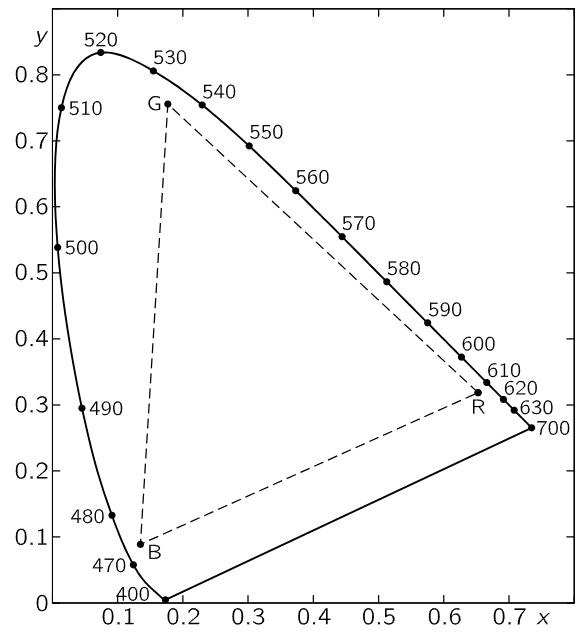
Fig. 35–4. The standard chromaticity diagram.

Now let us discuss the combination of colors on a mathematical level as a geometrical proposition. If any one color is represented by Eq. (35.4), we can plot it as a vector in space by plotting along three axes the amounts a, b, and c, and then a certain color is a point. If another color is a′, b′, c′, that color is located somewhere else. The sum of the two, as we know, is the color which comes from adding these as vectors. We can simplify this diagram and represent everything on a plane by the following observation: if we had a certain color light, and merely doubled a and b and c, that is, if we make them all stronger in the same ratio, it is the same color, but brighter. So if we agree to reduce everything to the same light intensity, then we can project everything onto a plane, and this has been done in Fig. 35–4. It follows that any color obtained by mixing a given two in some proportion will lie somewhere on a line drawn between the two points. For instance, a fifty-fifty mixture would appear halfway between them, and 1/4 of one and 3/4 of the other would appear 1/4 of the way from one point to the other, and so on. If we use a blue and a green and a red, as primaries, we see that all the colors that we can make with positive coefficients are inside the dotted triangle, which contains almost all of the colors that we can ever see, because all the colors that we can ever see are enclosed in the oddly shaped area bounded by the curve. Where did this area come from? Once somebody made a very careful match of all the colors that we can see against three special ones. But we do not have to check all colors that we can see, we only have to check the pure spectral colors, the lines of the spectrum. Any light can be considered as a sum of various positive amounts of various pure spectral colors—pure from the physical standpoint. A given light will have a certain amount of red, yellow, blue, and so on—spectral colors. So if we know how much of each of our three chosen primaries is needed to make each of these pure components, we can calculate how much of each is needed to make our given color. So, if we find out what the color coefficients of all the spectral colors are for any given three primary colors, then we can work out the whole color mixing table.

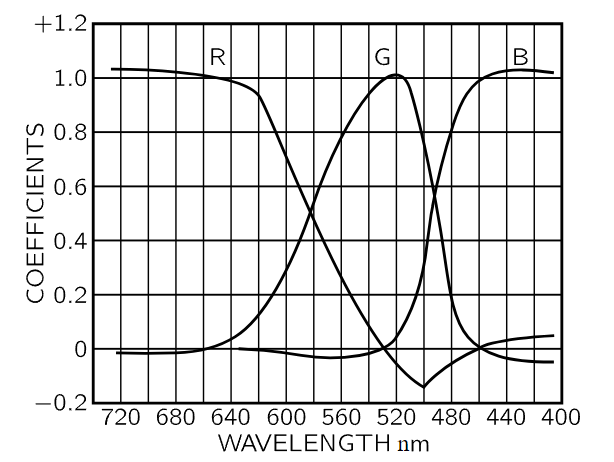
Fig. 35–5. The color coefficients of pure spectral colors in terms of a certain set of standard primary colors.

An example of such experimental results for mixing three lights together is given in Fig. 35–5. This figure shows the amount of each of three different particular primaries, red, green and blue, which is required to make each of the spectral colors. Red is at the left end of the spectrum, yellow is next, and so on, all the way to blue. Notice that at some points minus signs are necessary. It is from such data that it is possible to locate the position of all of the colors on a chart, where the x- and the y-coordinates are related to the amounts of the different primaries that are used. That is the way that the curved boundary line has been found. It is the locus of the pure spectral colors. Now any other color can be made by adding spectral lines, of course, and so we find that anything that can be produced by connecting one part of this curve to another is a color that is available in nature. The straight line connects the extreme violet end of the spectrum with the extreme red end. It is the locus of the purples. Inside the boundary are colors that can be made with lights, and outside it are colors that cannot be made with lights, and nobody has ever seen them (except, possibly, in after-images!).

مواضيع ذات صلة

The sensation of color

Physiochemistry of color vision

The mechanism of color vision

Measuring the color sensation

Color depends on intensity

Aberration

The ω,k four-vector

Moving sources

Anomalous refraction

The intensity of reflected light

Optical activity

Polarizers