We have qualitatively demonstrated that there are maxima and minima in the radiation field from two sources, and our problem now is to describe the field in mathematical detail, not just qualitatively.

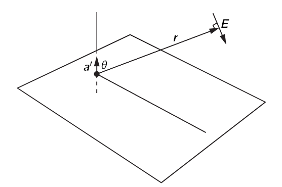
Fig. 29–1. The electric field E due to a positive charge whose retarded acceleration is a′.

We have already physically analyzed the meaning of formula (28.6) quite satisfactorily, but there are a few points to be made about it mathematically. In the first place, if a charge is accelerating up and down along a line, in a motion of very small amplitude, the field at some angle θ from the axis of the motion is in a direction at right angles to the line of sight and in the plane containing both the acceleration and the line of sight (Fig. 29–1). If the distance is called r, then at time t the electric field has the magnitude

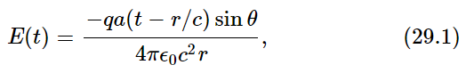
where a(t−r/c) is the acceleration at the time (t−r/c), called the retarded acceleration.

Now it would be interesting to draw a picture of the field under different conditions. The thing that is interesting, of course, is the factor a(t−r/c), and to understand it we can take the simplest case, θ=90^∘, and plot the field graphically. What we had been thinking of before is that we stand in one position and ask how the field there changes with time. But instead of that, we are now going to see what the field looks like at different positions in space at a given instant. So, what we want is a “snapshot” picture which tells us what the field is in different places. Of course, it depends upon the acceleration of the charge. Suppose that the charge at first had some particular motion: it was initially standing still, and it suddenly accelerated in some manner, as shown in Fig. 29–2, and then stopped. Then, a little bit later, we measure the field at a different place. Then we may assert that the field will appear as shown in Fig. 29–3. At each point the field is determined by the acceleration of the charge at an earlier time, the amount earlier being the delay r/c. The field at farther and farther points is determined by the acceleration at earlier and earlier times. So the curve in Fig. 29–3 is really, in a sense, a “reversed” plot of the acceleration as a function of time; the distance is related to time by a constant scale factor c, which we often take as unity. This is easily seen by considering the mathematical behavior of a(t−r/c). Evidently, if we add a little time Δt, we get the same value for a(t−r/c) as we would have if we had subtracted a little distance: Δr=−cΔt.

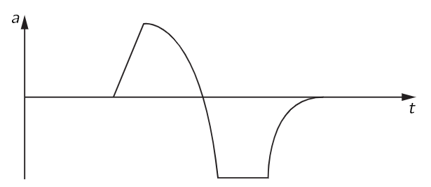
Fig. 29–2. The acceleration of a certain charge as a function of time.

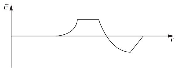
Fig. 29–3. The electric field as a function of position at a later time. (The 1/r variation is ignored.)

Stated another way: if we add a little time Δt, we can restore a(t−r/c) to its former value by adding a little distance Δr=cΔt. That is, as time goes on the field moves as a wave outward from the source. That is the reason why we sometimes say light is propagated as waves. It is equivalent to saying that the field is delayed, or to saying that the electric field is moving outward as time goes on.

An interesting special case is that where the charge q is moving up and down in an oscillatory manner. The displacement x at any time t was equal to a certain constant x₀, the magnitude of the oscillation, times cos ωt. Then the acceleration is

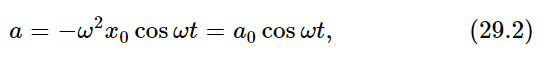
where a₀ is the maximum acceleration, −ω²x₀. Putting this formula into (29.1), we find

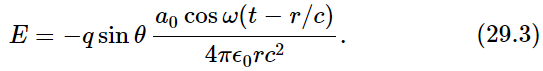
Now, ignoring the angle θ and the constant factors, let us see what that looks like as a function of position or as a function of time.

مواضيع ذات صلة

Mirror reflections

The sensation of color

Physiochemistry of color vision

The mechanism of color vision

The chromaticity diagram

Measuring the color sensation

Color depends on intensity

Aberration

The ω,k four-vector

Moving sources

Anomalous refraction

The intensity of reflected light